Analyze: How it works

Operation sequence

Analyze generates a reference signal and writes it as PCM Data to stdout, a file or a pipe.

At the same time it reads 2 channel PCM Data from stdin, a file or a pipe and does the analysis on the fly. The result is written to the file data.dat and/or the screen (stderr) every time new data is available.

Optionally a command could be executed or passed to stdout at several events. E.g. when new data is available to synchronize Gnuplot.

The program terminates, if the indicated number of turns has completed, no more input is available or an interrupt signal is received (Ctrl-C).

Almost any step in the program flow is optional. E.g. you might only generate a reference or only perform the analysis. And, of course, any event or file system write is optional.

Modes of operation

Analyze currently supports two operation modes

1. Noise mode (default)
   

   In this mode a reference with a well defined spectrum is used as reference.

2. Sweep mode (option msweep)
   

   In sweep mode all frequencies are measured after each other. The measurement terminates when the last frequency has completed.

   Each frequency measurement consists of a setup time (predelay) typically one FFT cycle followed by some FFT cycles for this frequency (ln). All frequencies in the result that do not match the current frequency (or one of its harmonics if enabled) are ignored. This acts like a lock-in filter and suppresses noise to a very high degree.

Logarithmic sweeps as recommended for measuring the impulse response of a room are currently not supported.

LCR analysis with PCA method (option mpca)

The PCA mode (Principal Component Analysis) uses a linear combination of the following functions to reproduce U(t) by I(t):

• a constant (DC offset, parasitic),
• R·I(t) (ohmic resistance),
• dI(t)/dt (inductance),
• ∫ I(t) dt (capacity) and
• x·t (drift of the DC offset, parasitic)

This is a very fast way to analyze a series of resistor, inductor and capacitor. The complexity is O(n) in the number of samples.
It works as long it is a series. You cannot measure the electrolytic capacitors this way, because there are other effects included.

The PCA method will not write a data file.

FFT and PCA can be combined. Then you will get the more reliable LCR values of the PCA method together with the detailed frequency dependent results from FFT in the data file.

FFT analysis (option mfft)

The FFT mode is intended for measurement of impedance and transfer functions. It calculates as follows:

$H\left(f\right)=\frac{Z\left(f\right)}{R_{\mathit{ref}}}=\frac{\mathrm{FFT}\left(L\left(t\right)\right)}{\mathrm{FFT}\left(R\left(t\right)\right)}$

with

input channel	two port measurement	impedance measurement
L(t)	response signal	voltage U(t)
R(t)	reference signal	current I(t)

Impedance measurement: ESR, ESC, ESL

ESR, ESC and ESL is calculated by fitting Z(f). Therefore the weighted averages in the interval [famin, famax] are calculated as follows:

ESR = < a_i > = < re(Z(f)) >
ESL = < b_i / ω > = < im(Z(f)) / ω >
ESC = < −b_i · ω > = < −im(Z(f)) · ω >

Of course, only one of ESL or ESC is reasonable, the positive one. The standard deviation of the above average values gives a coarse estimation of the reliability.

You will not get reasonable results when the impedance contains components that change with frequency. In this case you should view the frequency dependent results in the data file. Electrolytic capacitors tend to show such behavior.

Noise Reference

This program analyze generates cyclic noise patterns with adjustable properties, like energy distribution and relatively prime frequencies. The cyclic nature of the patterns makes the spectrum discrete which is ideal for FFT analysis without the need of a window function.

Energy distribution

The program creates the noise reference by inverse Discrete Fourier Transform. The amplitudes of the Fourier coefficients are calculated by:

r_i = f_i^κ

The phase angles are chosen randomly.

The exponent κ controls the energy distribution. An homogeneous distribution (κ = 0) represents white noise. Positive values prefer high frequencies, negative values prefer low frequencies. κ = -1 creates pink noise.

All coefficients, outside the frequency range [f_min, f_max], are purged. This is particularly required when κ < 0, because otherwise the amplitude of the DC component becomes singular.

After the Inverse Fourier Transform the wave form is normalized to 0dB FSR unless another level is selected by option gain.

Dealing with harmonics

The harmonics option excludes frequencies from the resulting spectrum if

• the current frequency is a harmonic of another used frequency or
• one of the first n harmonics of the current frequency is a harmonic of another used frequency.

Because of the second condition it is strongly recommended to set the minimum frequency at least higher than the nth harmonic of the ground frequency of the generated pattern. Otherwise a large gap would occur after the first used frequency.

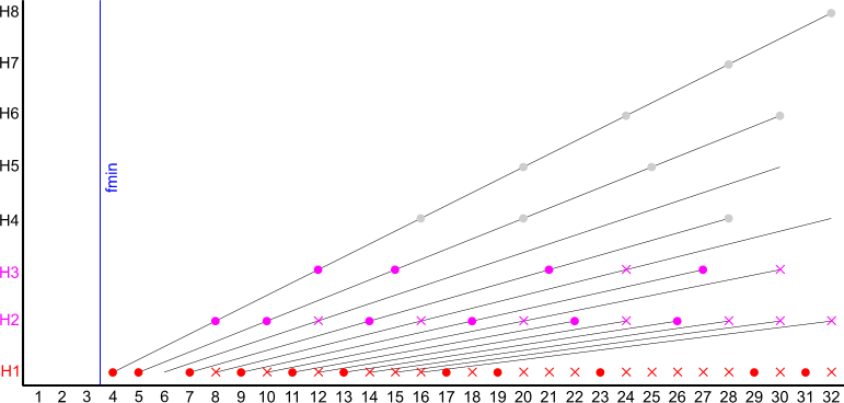
The graph shows an example of the generated frequencies for a 64 sample noise pattern with 3 harmonics and a minimum frequency of 4:

analyze fftlen=64 fsamp=64 fmin=3 fmax=32 harm3 wspec=noise.dat

Rationale

• Frequency 4 is the first after fmin. This is always used.
• Frequency 6 has a collision at its 2nd harmonic with the 3rd harmonic of frequency 4 at frequency 12 and therefore cannot be used because it would make frequency 12 ambiguous.
• Frequency 5 has also a collision at its 4th harmonic with the 5th harmonic of frequency 4, but both are beyond the maximum harmonic to analyze (3 in this case) and so this does not care.
• Frequency 8 has a direct collision with the 2nd harmonic of frequency 4 and must not be used.
• Frequency 16 has a direct collision with the 4th harmonic of frequency 4. Although this harmonic is not analyzed it might get additional energy by non-linearities, so it is not used either.

In effect the noise pattern contains only energy at the frequencies with red circles. While all the frequencies with red or pink circles are used for analysis.

Two channel mode

In two channel mode Analyze generates distinct reference signals for the left and the right output. In fact every second usable frequency is sent to the 2nd channel while the other frequencies are sent to the left channel.

This is intended for fast room measurements. You can get the frequency response of both speakers at once. Since the references are orthogonal you can simply plot left and right channel data in a different graph. Of course, you loose some accuracy but for a coarse characterization e.g. to adjust an equalizer this is enough.