Analyze: Calibration

Overview

Calibration can significantly improve the accuracy of the measurements. Analyze supports 3 levels of calibration:

1. One point calibration
   

   This method only compensates for differences of the left and right channel of the sound device. In most cases that adds no much value since most sound devices have no significant differences here. Therefore this method is not recommended unless you want to compensate for additional external components.

2. Two point matrix calibration
   

   This calibration compensates for cross talk. While cross talk is no serious issue in most sound devices it might be considerably in measurement setups. If your setup has a stable reference signal, i.e. independent of the measurement sample load and you do not use a 4 point probe, than this kind of calibration is usually sufficient. This applies typically to two port measurements of transfer functions with an very low output impedance amplifier as source, e.g. an audio amplifier.

3. Three point matrix calibration
   

   This compensates for all relevant linear deviations of the measurement setup. Strictly speaking there is a forth degree of freedom in the matrix, but since absolute amplitudes do not count in all supported measurement modes there is no need for a full calibration.
   Three point calibration is recommended for impedance measurements with 4 point probes.

All kinds of calibrations are frequency dependent and complex, i.e. compensate for amplitude and phase of each frequency.

General rules

• It is essential that the sampling rate of the DAC exactly matches that of the ADC, i.e they have to use the same clock oscillator. This requirement is usually fulfilled if and only if both are on the same sound device.
  
• The sampling rate used for calibration should match the sampling rate used for measurements. While it is possible to measure at lower sampling rates adaptive aliasing filters of the sound device might impact the result.
• The FFT size need not to match. Since the coefficients of the correction matrix show only moderate frequency dependency it is just fine to use a smaller FFT size for calibration to reduce noise.

Gain correction

The simple gain calibration mode only takes care of the differences in the transfer function between the two input channels. This is sufficient to compensate for tolerances and phase differences between the channels. This is particularly important in differential mode.

Note that the gain calibration does not compensate for the absolute transfer function of the sound device in any way. It does not even distinguish between the transfer function of the line output stage and the transfer function of the line input.

How to do gain calibration

Connect both line in channels to one line out channel. Play a white noise and activate the gain correction mode with option gg.

Result

Example of gain correction: Terratec XLerate (Aureal AU8820 chip) at 48kHz and an FFT length of 65536 samples, average over 10 cycles.
The deviation in the amplitude is with < 0,2 dB pretty good, but the channels are obviously not sampled simultaneously. The time difference of ½ sample at the Nyquist frequency point to a serial conversion with two way oversampling.

The result of the gain calibration is the complex and frequency dependent quotient:

$\mathit{gain\_corr}\left(f\right)=\frac{\mathrm{FFT}\left(\mathit{channel\; 2}\right)}{\mathrm{FFT}\left(\mathit{channel\; 1}\right)}$

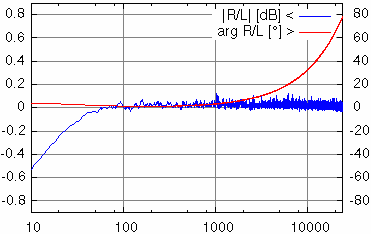
The magnitude of this quotient is a measure of the degree of gain difference between the two channels. A typical value is mainly independent of the frequency and close to but not exactly one. This is due to tolerances in resistors. At low frequencies the difference may increase due to tolerances in the coupling capacitors.

The phase angle of the correction shows the synchronization of the channels. Beyond the small differences due to tolerance of the coupling capacitors there are usually no particular deviations. But some sound devices sample the two channels not simultaneously but alternating. In this case there is a linear phase shift.

Using the correction

When using the correction is used with option gr it is applied to both channels symmetrically.

$\mathrm{FFT}\left(\mathit{channel\; 1\text{'}}\right)=\mathrm{FFT}\left(\mathit{channel\; 1}\right)·\sqrt{\mathit{gain\_corr}\left(f\right)}$
$\mathrm{FFT}\left(\mathit{channel\; 2\text{'}}\right)=\mathrm{FFT}\left(\mathit{channel\; 2}\right)/\sqrt{\mathit{gain\_corr}\left(f\right)}$

Do not use this correction to compensate for a complex transition function or there will be an impact on automatic weight function.

Matrix correction

The simple gain calibration method above does not compensate for cross talk. So there is a superior calibration method called matrix calibration. It should be preferred at least for impedance measurements.

Using $L_{\mathrm{ideal}}\propto U$ and $R_{\mathrm{ideal}}\propto I·R_{\mathrm{ref}}$ (L = channel 1, R = channel 2) the real impedance is:

$Z=\left[\begin{array}{c}{L}_{\mathrm{ideal}}\\ R_{\mathrm{ideal}}\end{array}\right]·R_{\mathrm{ref}}$

But in fact you can't see L_ideal and R_ideal. What you really record is L_real and R_real, a transformation:

$\left[\begin{array}{c}{L}_{\mathrm{real}}\\ R_{\mathrm{real}}\end{array}\right]=\left[\begin{array}{c}{L}_{\mathrm{ideal}}\\ R_{\mathrm{ideal}}\end{array}\right]·\left[\begin{array}{cc}{c}_{\mathrm{ll}}& c_{\mathrm{rl}}\\ c_{\mathrm{lr}}& c_{\mathrm{rr}}\end{array}\right]$

Of course, all the coefficients c_xx are complex and frequency dependent.

Using the matrix correction

The matrix correction is applied to the measurement data with option zr. This calculates the inverse transformation matrix and applies it to the input data before the data is passed to the FFT analysis.

$\left[\begin{array}{c}{L}_{\mathrm{ideal}}\\ R_{\mathrm{ideal}}\end{array}\right]=\left[\begin{array}{c}{L}_{\mathrm{real}}\\ R_{\mathrm{real}}\end{array}\right]·{\left[\begin{array}{cc}{c}_{\mathrm{ll}}& c_{\mathrm{rl}}\\ c_{\mathrm{lr}}& c_{\mathrm{rr}}\end{array}\right]}^{-1}$

The sampling rate and the FFT size of the matrix correction data do not need to match the values of the current measurement. A linear interpolation is used in doubt. But it is recommended to match the sampling rate matches because sound devices tend to have sampling rate dependent filtering and the interpolation is very simple.

2 point matrix calibration

The easiest way to get the calibration coefficients is a two point calibration. This mode is activated by the zg zn options.

It basically does

• one measurement with L_ideal = 0 and
• one measurement with R_ideal = 0.

This is, of course, not sufficient to get four coefficients. So further assumptions are needed. The main assumption is that the sum of L_real + R_real is the same for both calibration measurements, i.e. the reference is the same.

$c_{\mathrm{ll}}+c_{\mathrm{rl}}=1$
$c_{\mathrm{lr}}+c_{\mathrm{rr}}=1$

While this is typically a good assumption for two port measurements it might be a bad one for impedance measurements due to wire inductance.

Calibration setup

Schematic how to prepare for matrix calibration of measurements of transfer functions.

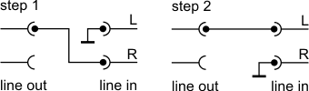
The first calibration is done with the reference signal only connected to channel 2 (R) and channel 1 (L) grounded. The second calibration is done the other way around.

If you use additional preamplifiers you should put the ground to their input instead of the sound devices input to compensate for their properties as well.

Calibration sequence

When the matrix calibration is initiated with option zg, analyze takes the following steps in sequence:

1. Discard the first samples. (option psa)
2. Record n cycles (option ln) of data.
3. Output a message to setup for the next step to stderr.
4. Discard some cycles. (option lp)
   In this time you have to change the setup for step two.
5. Record another n cycles.
6. Write the result file (option zg) and terminate.

Important notes

It is essential to use absolutely the same reference signal in both steps. The reference therefore must be exactly reproducible. So it cannot be done with white noise but must by cyclic. This implies to use the same output channel of the sound device, too. It is also essential the the phase of the reference signal is 100% correlated in both steps. This is the reason why both measurements have to be done at one single run without closing the sound device in between. The synchronization of the input (ADC) and the output (DAC) have to be stable within less than one sample over the whole measurement. This is only possible if both are controlled by the same crystal oscillator. Fortunately this is naturally ensured as long as both ports are on the same sound device.

Result

In theory the matrix correction omits all linear errors without the need of an absolute reference. Practically this only works for the correction of sound device itself. For impedance measurements there is one degree of freedom to much. You know neither R_ideal at Z = 0 nor L_ideal at Z = ∞ and they are not necessarily the same. You could eliminate the additional degree of freedom if you assume that U_ref ∝ L_ideal + R_ideal => R_ideal at Z = 0 equals L_ideal at Z = ∞ (see option zn). But this introduces the systematic error that the high current at Z = 0 causes an additional voltage drop at inductance of the wires.

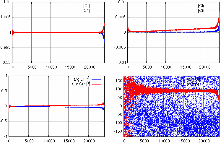Example of matrix calibration result: on board Realtek ALC650 codec at 48 kHz sampling rate and a self-made probe with 200Ω R_ref and an FFT length of 65536 samples, averaged over 10 cycles.
The graphs show the diagonal (left) and the non diagonal (right) matrix elements, each with amplitude (top) and phase angle in degrees (bottom).
You see a capacitive cross talk from channel 1 to channel 2. The asymmetric cross talk is due to the probe.
The phase response of c_ll and c_rr shows a delay of about 12ns (!) between both channels. Note the extremely high accuracy in spite of the 20µs sampling resolution.
c_lr is that small (about -70 dB) that its phase (blue) is nearly undetermined.

3 Point matrix calibration

Three point calibration is primarily intended for impedance measurements, but it may be used for two port measurements as well. It will use a third calibration measurement with a known impedance (or a known transfer function respectively). This compensates for all linear deviations.

Calibration sequence

When the 3 point matrix calibration is initiated with option zg, analyze takes the following steps in sequence:

1. Discard the first samples. (option psa)
2. Record n cycles (option ln) of data for the reference impedance, Z = 1 by default.
3. Output a message to setup for the next step to stderr.
4. Discard some cycles. (option lp)
   In this time you have to change the setup for step two.
5. Record another n cycles for impedance Z = 0.
6. Output a message to setup for the next step to stderr.
7. Discard some cycles. (option lp)
   In this time you have to change the setup for step three.
8. Record the last n cycles for impedance Z = ∞.
   
9. Write the result file (option zg) and terminate.

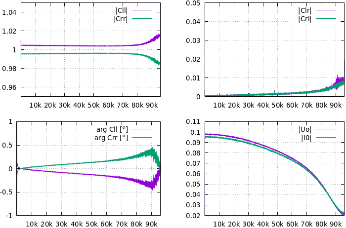Example of 3 point matrix calibration of on-board Intel HDA device with 192 kHz sampling rate and a self-made probe with 20 Ω reference resistor.
The about 0,5 % gain difference (Cll vs Crr) is due to an inexact reference resistor. Additionally there is a slight cross-talk. The decrease of the absolute amplitude at higher frequencies is due to the used simple external audio equipment that was not intended for frequencies beyond 20 kHz. Nevertheless results up to approximately 60 kHz are reliable after calibration.